Constraint Based Analysis with PSAMM
This tutorial will go over how to use the constraint based analysis methods that are included in PSAMM. These methods can be used to perform various simulations of growth with metabolic models. These simulations can be used to explore growth phenotypes, nutrient utilization, and gene essentiality.
Tutorial Materials
The materials used in the part of the tutorial can be found in the tutorial-part-3 directory in the psamm-tutorial repository. This directory contains a copy of the E. coli core metabolic model that has been used in the other tutorials. This model can be used to run all of the simulations in this part of the tutorial. In addition to the model the virtual environment where PSAMM has been installed will need to be activated to run the psamm-model commands. For instructions on how to install or activate PSAMM in a virtual environment reference the Installation and Materials section of the tutorial.
To access the materials needed to run the following commands go to the E_coli_yaml folder in the tutorial-part-3 folder.
(psamm-env) $ cd <PATH>/tutorial-part-3/E_coli_yaml
Constraint-based Flux Analysis with PSAMM
Along with the various curation tools that are included with PSAMM there are also various flux analysis tools that can be used to perform simulations on the model. This allows for a seamless integration of the model development, curation, and simulation processes.
There are various options that you can change in these different flux analysis commands. Before introducing the specific commands these options will be detailed here.
Loop Minimization in PSAMM
First, you can choose the options for loop minimization when running
constraint-based analyses. This can be done by using the --loop-removal
option. There are three options for loop removal when performing constraint
based analysis:
- none
- No removal of loops
- tfba
- Removes loops by applying thermodynamic constraints
- l1min
- Removes loops by minimizing the L1 norm (the sum of absolute flux values)
For example, you could run flux balance analysis with thermodynamic constraints:
(psamm-env) $ psamm-model fba --loop-removal=tfba
or without:
(psamm-env) $ psamm-model fba --loop-removal=none
Choosing Linear Programming Solvers
You also have the option to set which solver you want to use for the linear programming problems. To view the solvers that are currently installed the following command can be used:
(psamm-env) $ psamm-list-lpsolvers
By default PSAMM will use CPLEX if it available but if you want to
specify a different solver you can do so using the --solver option. For
example to select the Gurobi solver during an FBA simulation you can use the
following command:
(psamm-env) $ psamm-model fba --solver name=gurobi
If multiple solvers are installed and you do not want to use the default solver, you will need to set this option for every simulation run.
Note
The QSopt_ex solver does not support integer linear programming problems. This solver can be used with any commands but you will not be able to run the simulation with thermodynamic constraints.
Other Global Options
Another option that can be used with the various flux analysis commands is the
--epsilon option. This option can be used to set the minimum value that a
flux needs to be above to be considered non-zero. By default PSAMM will
consider any number above \(10^{-5}\) to be non-zero. An example of
changing the epsilon value with this option during an FBA simulation is:
(psamm-env) $ psamm-model fba --epsilon 0.0001
These various options can be used for any of the flux analysis functions in PSAMM by adding them to the command that is being run. A list of the functions available in PSAMM can be viewed by using the command:
(psamm-env) $ psamm-model --help
The options for a specific function can be viewed by using the command:
(psamm-env) $ psamm-model <command> --help
FBA in PSAMM
PSAMM allows for the integration of the model development and curation process with the simulation process. In this way changes to a metabolic model can be immediately tested using the various flux analysis tools that are present in PSAMM. In this tutorial, aspects of the E. coli core model [Orth11] will be expanded to demonstrate the various functions available in PSAMM and throughout these changes the model will be analyzed with PSAMM’s simulation functions to make sure that these changes are resulting in a functional model.
Flux Balance Analysis
Flux Balance Analysis (FBA) is one of the basic methods that allows you
to quickly examine if the model is viable (i.e. can produce biomass). PSAMM
provides the fba function in the psamm-model command to perform FBA on
metabolic models. For example, to run FBA on the E. coli core model first
make sure that the current directory is the E_coli_yaml/ directory using
the following command:
(psamm-env) $ cd <PATH>/psamm-tutorial/E_coli_yaml/
Then run FBA on the model with the following command.
(psamm-env) $ psamm-model fba
Note that the command above should be executed within the folder that stores
the model.yaml file. Alternatively, you could run the following command anywhere
in your file system:
(psamm-env) $ psamm-model --model <PATH-TO-MODEL.YAML> fba
The following is a sample of some output from the FBA command:
INFO: Model: Ecoli_core_model
INFO: Model Git version: 9812080
INFO: Using Biomass_Ecoli_core_w_GAM as objective
INFO: Loop removal disabled; spurious loops are allowed
INFO: Setting feasibility tolerance to 1e-09
INFO: Setting optimality tolerance to 1e-09
INFO: Solving took 0.05 seconds
ACONTa      6.00724957535   |Citrate[c]| <=> |cis-Aconitate[c]| + |H2O[c]|  b0118 or b1276
ACONTb      6.00724957535   |cis-Aconitate[c]| + |H2O[c]| <=> |Isocitrate[c]|       b0118 or b1276
AKGDH       5.06437566148   |2-Oxoglutarate[c]| + |Coenzyme-A[c]|...
...
INFO: Objective flux: 0.873921506968
INFO: Reactions at zero flux: 47/95
At the beginning of the output of psamm-model commands information about
the model as well as information about simulation settings will be printed.
At the end of the output PSAMM will print the maximized flux of the designated
objective function. The rest of the output is a list of the reaction IDs in the
model along with their fluxes,
and the reaction equations represented with the compound names. This output is
human readable because the reactions equations are represented with the full
names of compound. It can be saved as a tab separated file that can be sorted
and analyzed quickly allowing for easy analysis and comparison between FBA in
different conditions.
By default, PSAMM fba will use the biomass function designated in the central
model file as the objective function. If the biomass tag is not defined in a
model.yaml file or if you want to use a different reaction as the
objective function, you can simply specify it using the --objective option.
For example to maximize the citrate synthase reactions, CS, the command would
be as follows:
(psamm-env) $ psamm-model fba --objective=CS
Flux balance analysis will be used throughout this tutorial as both a checking tool during model curation and an analysis tool. PSAMM allows you to easily integrate analysis tools like this into the various steps during model development.
Flux Variability Analysis
Another flux analysis tool that can be used in PSAMM is flux variability analysis. This analysis will maximize the objective function that is designated and provide a lower and upper bound of the various reactions in the model that would still allow the model to sustain the same objective function flux. This can provide insights into alternative pathways in the model and allow the identification of reactions that can vary in use.
To run FVA on the model use the following command:
(psamm-env) $ psamm-model fva
...
EX_pi_e     -3.44906664664  -3.44906664664  |Phosphate[e]| <=>
EX_pyr_e    -0.0    -0.0    |Pyruvate[e]| <=>
EX_succ_e   -0.0    -0.0    |Succinate[e]| <=>
FBA 7.00227721609   7.00227721609   |D-Fructose-1-6-bisphosphate[c]| <=> |Dihydroxyacetone-phosphate[c]| + |Glyceraldehyde-3-phosphate[c]|
FBP 0.0     0.0     |D-Fructose-1-6-bisphosphate[c]| + |H2O[c]| => |D-Fructose-6-phosphate[c]| + |Phosphate[c]|
FORt2       0.0     0.0     |Formate[e]| + |H[e]| => |Formate[c]| + |H[c]|
...
The output shows the reaction IDs in the first column and then shows the lower bound of the flux, the upper bound of the flux, and the reaction equations. With the current conditions the flux is not variable through the equations in the model. It can be seen that the upper and lower bounds of each reaction are the same. If another carbon source was added in though it would allow for more reactions to be variable. For example if glucose was added into the media along with mannitol then the results might appear as follows:
EX_glc_e    -10.0   -2.0    |D-Glucose[e]| <=>
EX_manni_e  -9.0    -3.0    |Mannitol[e]| <=>
MANNIPTS    3.0     9.0     |Mannitol[e]| + |Phosphoenolpyruvate[c]| => |Mannitol 1-phosphate[c]| + |Pyruvate[c]|
GLCpts      2.0     10.0    |D-Glucose[e]| + |Phosphoenolpyruvate[c]| => |Pyruvate[c]| + |D-Glucose-6-phosphate[c]|
It can be seen that in this situation the lower and upper bounds of some reactions are different indicating that their flux can be variable. This indicates that there is some variability in the model as to how certain reactions can be used while still maintaining the same objective function flux.
Robustness Analysis
Robustness analysis can be used to analyze the model under varying conditions. Robustness analysis will maximize a designated reaction while varying the flux through another designated reaction. For example, you could vary the amount of oxygen present while trying to maximize the biomass production to see how the model responds to different oxygen supply. You can specify the number of steps that will be performed in the robustness as well as the reaction that will be varied during the steps.
By default, the reaction that is maximized will be the biomass reaction defined
in the model.yaml file but a different reaction can be designated
with the optional --objective option. The flux bounds of this reaction will
then be obtained to determine the lower and upper value for the robustness
analysis. These values will then be used as the starting and stopping points
for the robustness analysis. You can also set a customized upper and lower flux
value of the varying reaction using the --lower and --upper options.
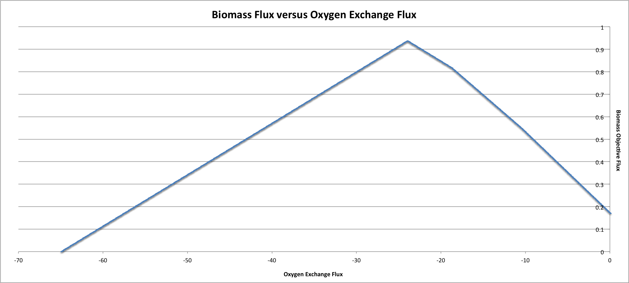
For this model the robustness command will be used to see how the model responds to various oxygen conditions with mannitol as the supplied carbon source. To run the robustness command use the following command:
(psamm-env) $ psamm-model robustness --steps 1000 EX_o2_e
The output will contain two columns. The first column will be the flux of the varied reaction, in this case the EX_o2_e reaction for oxygen exchange. The second shows the flux of the biomass reaction for the model. The output will look like this:
-63.958958959       0.0238161275506
-63.8938938939      0.0253046355225
-63.8288288288      0.0267931434944
-63.7637637638      0.0282816514663
-63.6986986987      0.0297701594383
-63.6336336336      0.0312586674102
-63.5685685686      0.0327471753821
-63.5035035035      0.034235683354
-63.4384384384      0.0357241913259
...
If the biomass reaction flux is plotted against the oxygen uptake it can be seen that the biomass flux is low at the highest oxygen uptake, reaches a maximum at an oxygen uptake of about 24, and then starts to decrease with low oxygen uptake.
If a more detailed analysis of internal fluxes is desired the –all-reaction-fluxes tag can be added to the command. This will print out all of the internal reaction fluxes for each step in the robustness analysis. The first column printed will be the reaction ID. The second column will be the varying reaction’s flux and the last column will be the flux of the reaction listed in the first column. This can be used to look at the effects of a reaction on internal fluxes in the network. The command to run this would be the following:
(psamm-env) $ psamm-model robustness --all-reaction-fluxes --steps 1000 EX_o2_e
And the output for this command will look like the following:
G6PDH2r     -63.958958959   0.0
AKGDH       -63.958958959   0.0
GLNS        -63.958958959   0.00608978381469
ADK1        -63.958958959   0.0
PYRt2r      -63.958958959   0.0
EX_co2_e    -63.958958959   58.986492784
ATPM        -63.958958959   8.39
SUCCt2_2    -63.958958959   0.0
PIt2r       -63.958958959   0.0876123884204
EX_lac_D_e  -63.958958959   0.0
Deletion Simulations with PSAMM
Gene Deletion
The genedelete command can be used to perform gene deletions in a model and test what effects those
deletions have. This command can be used to quickly test if certain genes are essential in the network. The
command will take a list of genes in a separate file and will then go through all of the gene associations in
the model to determine what reactions require that gene to be present. This uses the gene association logic
to determine if the removal of the specified genes would knock out that function. For example if we had the
following two reactions:
- id: RXN_1
  genes: g0001 and g0002
  equation: '|cpd_a[c]| <=> |cpd_b[c]|'

- id: RXN_2
  genes: g0001 or g0003
  equation: '|cpd_a[c]| <=> |cpd[c]|'
Both reactions are associated with the gene ‘g0001’ but RXN_1 has an ‘and’ association while RXN_2 has an ‘or’ association. If the gene ‘g0001’ were to be deleted from the network RXN_1 would no longer have the required genes for it to be present since both genes are required. RXN_2 would still be satisfied since it would only require one of the two genes to be present. The gene delete command will do this automatically and for the entire network making it much easier to do these kinds of simulations. The gene delete command can be run with the following command.
(psamm-env) $ psamm-model genedelete --gene b1779
This will produce a flux balance analysis result with a model that has any reactions for which b0118 is necessary limited to zero flux. The output will show a percentage of the biomass flux of the wild type model that can be produced by the deletion model.
...
INFO: Objective reaction after gene deletion has flux 0.0
INFO: Objective reaction has 0.00% flux of wild type flux
Random Minimal Network Analysis
The randomsparse command can
be used to look at gene essentiality in the metabolic network. To use this function
the model must contain gene associations for the model reactions. This
function works by systematically deleting genes from the network, then
evaluating if the associated reaction would still be available after
the gene deletion, and finally testing the new network to see if the
objective function flux is still above the threshold for viability.
If the flux falls too low then the
gene is marked as essential and kept in the network. If the flux stays
above the threshold then the gene will be marked as non-essential and
removed. The program will randomly do this for all genes until the only
ones left are marked as essential. This can be
done using the --type=genes option with the randomsparse command:
(psamm-env) $ psamm-model randomsparse --type=genes 90%
This will produce an output of the gene IDs with a 1 if the gene was kept in the simulation and a 0 if the gene was deleted. Following the list of genes will be a summary of how many genes were kept out of the total as well as list of the reaction IDs that made up the minimal network for that simulation. An example output can be seen as follows:
INFO: Essential genes: 58/137
INFO: Deleted genes: 79/137
b0008       0
b0114       1
b0115       1
b0116       1
b0118       0
b0351       0
b0356       0
b0451       0
b0474       0
b0485       0
...
The random minimal network analysis can also be used to generate a random
subset of reactions from the model that will still allow the model to
maintain an objective function flux above a user-defined threshold. This
function works on the same principle as the gene deletions but instead of
removing individual genes, reactions will be removed.
To run random minimal network analysis on the
model use the randomsparse command with the --type=reactions option. The
last parameter for the command is a percentage of the maximum objective flux
that will be used as the threshold for the simulation.
(psamm-env) $ psamm-model randomsparse --type=reactions 95%
...
FRUKIN      1
...
MANNI1PDEH  0
MANNI1PPHOS 1
MANNIDEH    1
MANNIPTS    1
...
The output will be a list of reaction IDs with either a 1 indicating that the reaction was essential or a zero indicating it was removed.
Due to the random order of deletions during this simulation it may be helpful to run this command numerous times in order to gain a statistically significant number of datapoints from which a minimal essential network of reactions can be established.
In this case the program deleted the MANN1PDEH reaction blocking the mannitol 1-phosphate to fructose 6-phosphate conversion. In this case the reactions in the other side of the mannitol utilization pathway should all be essential.
You can also use the randomsparse command to randomly sample the exchange
reactions and generate putative minimal exchange reaction sets. This can be
done by using the --type=exchange option with the randomsparse command:
(psamm-env) $ psamm-model randomsparse --type=exchange 90%
It can be seen that when this is run on this small network the mannitol exchange as well as some other small molecules are identified as being essential to the network:
EX_ac_e     0
EX_acald_e  0
EX_akg_e    0
EX_co2_e    1
EX_etoh_e   0
EX_for_e    0
EX_fru_e    0
EX_fum_e    0
EX_glc_e    0
EX_gln_L_e  0
EX_glu_L_e  0
EX_h2o_e    1
EX_h_e      1
EX_lac_D_e  0
EX_mal_L_e  0
EX_manni_e  1
EX_nh4_e    1
EX_o2_e     1
EX_pi_e     1
EX_pyr_e    0
EX_succ_e   0