Reactant/Product Pair Prediction and Visualization Using FindPrimaryPairs

This tutorial will go over how to use the primarypairs and PSAMM-Vis functions in PSAMM. These functions can be used to predict reactant/product pairs in metabolic models and to use these predictions to generate visualizations of metabolic networks.

Materials

For information on how to install PSAMM and the associated requirements, as well how to download the materials required for this tutorial, you can reference the Installation and Materials section of the tutorial.

In addition to the basic installation of PSAMM, the visualization function uses the Graphviz program to generate images from the text-based graph format produced by the vis command. Graphviz version > 0.8.4 must be installed along with the Graphviz python bindings.

Note

Graphviz download: https://www.graphviz.org/download/

Graphviz python bindings: https://pypi.org/project/graphviz/ or (psamm-env) $ pip install graphviz

For this part of the tutorial, we will be using a modified version of the E. coli core metabolic model that has been used in the other sections of the tutorial. This model has been modified to add in a new pathway for the utilization of mannitol as a carbon source. To access this model and the other files needed you will need to go into the tutorial-part-4 folder located in the psamm-tutorial folder.

(psamm-env) $ cd <PATH>/tutorial-part-4/

Once in this folder, you should see a folder called E_coli_yaml which contains all of the required model files, and a directory called additional_files/ that contains additional input files that will be used to run the commands in this tutorial.

To run the following tutorials, go into the E_coli_yaml/ directory:

(psamm-env) $ cd E_coli_yaml/

Reactant/Product Pair Prediction using PSAMM

Metabolism can be broken down into individual metabolic reactions, which transfer elements between different metabolites. Take the following reaction as an example:

Acetate + ATP <=> Acetyl-Phosphate + ADP

This reaction is catalyzed by the enzyme Acetate Kinase, which can convert acetate to acetyl-phosphate through the addition of a phosphate group from ATP. A basic understanding of phosphorylation and the biological role of ATP makes it possible to manually predict that the primary element transfers for non hydrogen elements are as follows:

Reactant/Product Pair	Element Transfer
Acetate -> Acetyl-Phosphate	carbon backbone
ATP -> ADP	carbon backbone and phosphates
ATP -> Acetyl-Phosphate	phosphate group
Acetate -> ADP	None

While manually inferring this for one or two simple reactions is possible, genome scale models often contain hundreds or thousands of reactions, making manual reactant/product pair prediction impractical. In addition to this, reaction mechanisms are often not known, nor are patterns of element transfer within reactions available for most metabolic reactions.

To address this problem the FindPrimaryPairs algorithm [Steffensen17] was developed and implemented within the PSAMM function primarypairs.

The FindPrimaryPairs is an iterative algorithm which is used to predict element transferring reactant/product pairs in genome scale models. FindPrimaryPairs relies on two sources of information, which are generally available in genome scale models: reaction stoichiometry and metabolite formulas. From this information, FindPrimaryPairs can make a global prediction of element transferring reactant/product pairs without any additional information about reaction mechanisms.

Basic Use of the primarypairs Command

The primarypairs command in PSAMM can be used to perform an element transferring pair prediction using the FindPrimaryPairs algorithm. The basic command can be run as the following:

(psamm-env) $ psamm-model primarypairs --exclude @../additional_files/exclude.tsv

This function often requires a file to be provided through the --exclude option. This file is a single column list of reaction IDs of any reactions the user wants to remove from the model when doing the reactant/product pair prediction. the file path should be included in the command with a ‘@’ preceding it. Typically, this file should contain any artificial reactions that might be in the model such as Biomass objective reactions, macromolecule synthesis reactions, etc. While these reactions can be left in the model, the fractional stoichiometries and presence of artificial metabolites in the reaction can cause the algorithm to take a much longer time to find a solution. In this example of the E. coli core model the only reaction like this is the biomass reaction Biomass_Ecoli_core_w_GAM, which this is the only reaction listed in the exclude.tsv file.

Note

The FindPrimaryPairs algorithm relies on metabolite formulas to make its reactant/product pair predictions. If any reaction contains a metabolite that does not have a formula then it will be ignored.

The output of the above command will look like the following:

INFO: Model: Ecoli_core_model
INFO: Model version: 3ac8db4
INFO: Using default element weights for fpp: C=1, H=0, *=0.82
INFO: Iteration 1: 79 reactions...
INFO: Iteration 2: 79 reactions...
INFO: Iteration 3: 8 reactions...
GLNS    nh4_c[c]        h_c[c]  H
FBA     fdp_c[c]        g3p_c[c]        C3H5O6P
ME2     mal_L_c[c]      nadph_c[c]      H
MANNI1PDEH      manni1p[c]      nadh_c[c]       H
PTAr    accoa_c[c]      coa_c[c]        C21H32N7O16P3S
....

Basic information about the model name and version is provided in the first few lines. In the next line, the element weights used by the FindPrimaryPairs algorithm are listed. Then, as the algorithm goes through multiple iterations, it will print out the iteration number and how many reactions it is still figuring out the pairing for. A four column table is then printed out that contains the following columns from left to right: Reaction ID, reactant ID, product ID, and elements transferred.

From this output, the Acetate Kinase reaction from the above example can be compared to the manual prediction of the element transfer. The reaction ID for this reaction is ACKr:

ACKr    atp_c[c]        adp_c[c]        C10H12N5O10P2
ACKr    atp_c[c]        actp_c[c]       O3P
ACKr    ac_c[c] actp_c[c]       C2H3O2

From this result it can be seen that the prediction contains the same three element transferring pairs as the above manual prediction; ATP -> ADP, ATP -> Acetyl-Phosphate, Acetate to Acetyl-Phosphate.

This basic usage of the primarypairs command allows for quick and accurate prediction of element transferring pairs in any of the reactions in a genome scale model. Additionally, the function also has a few other options that can be used to refine and adjust how the pair prediction work.

Modifying Element Weights

The metabolite pair prediction relies on a parameter called element weight to inform the algorithm about what chemical elements should be considered more or less important when determining metabolite similarity. An example of how this might be used can be seen in the default element weights that are reported when running primarypairs.

INFO: Using default element weights for fpp: C=1, H=0, *=0.82

These element weights are the default weights used when running primarypairs with the FindPrimaryPairs algorithm. In this case, a weight of 1 is given to carbon. Because carbon forms the structural backbone of many metabolites this element is given the most weight. In contrast, hydrogen is not usually a major structural element within metabolites. This leads to a weight of 0 being given to hydrogen, meaning that it is not considered when comparing formulas between two metabolites. By default, all other elements are given an intermediate weight of 0.82.

These default element weights can be adjusted using the --weights command line argument. For example, to adjust the weight of the element nitrogen while keeping the other elements the same as the default settings, you could use the following command:

(psamm-env) $ psamm-model primarypairs --weights "N=0.2,C=1,H=0,*=0.82" --exclude @../additional_files/exclude.tsv

In the case of a small model like the E. coli core model, the results of primarypairs will likely not change unless the weights are drastically altered. However, changes could be seen in larger models, especially if the models include many reactions related to non-carbon metabolism such as sulfur or nitrogen metabolism.

Report Element

By default, the primarypairs result is not filtered to show transfers of any specific element. In certain situations it might be desirable to only get a subset of these results based on if the reactant/product pair transfers a target element. To do this, the option --report-element can be used. In many cases, it might be desirable to only report carbon transferring reactant/product pairs, to do this run the following on the E. coli model.

(psamm-env) $ psamm-model primarypairs --report-element C --exclude @../additional_files/exclude.tsv

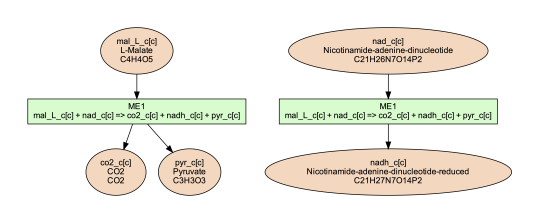
If the predicted pairs are looked at for one of the mannitol pathway reactions, MANNIDEH, the following can be seen:

MANNIDEH        manni[c]        fru_c[c]        C6H12O6
MANNIDEH        nad_c[c]        nadh_c[c]       C21H26N7O14P2

If this result is compared to the results without the --report-element C option, it can be seen that when there are additional transfers in this reaction, but they only involve hydrogen.

MANNIDEH        manni[c]        nadh_c[c]       H
MANNIDEH        manni[c]        h_c[c]  H
MANNIDEH        manni[c]        fru_c[c]        C6H12O6
MANNIDEH        nad_c[c]        nadh_c[c]       C21H26N7O14P2

Pair Prediction Methods

Two reactant/product pair prediction algorithms are implemented in the PSAMM primarypairs command. The default algorithm is the FindPrimaryPairs algorithm. The other algorithm that is implemented is the Mapmaker algorithm. These algorithms can be chosen through the --method argument.

$ psammm-model primarypairs --method fpp
or
$ psamm-model primarypairs --method mapmaker

Visualizing Models using PSAMM-Vis

PSAMM-Vis, as implemented in the vis command in PSAMM, can be used to convert text-based YAML models to graph-based representations of the metabolism. The graph-based representation contains two sets of nodes: one set representing the metabolites in the model and one set representing reactions. These nodes are connected through edges that are determined based on element transfer patterns predicted through using the FindPrimaryPairs algorithm. The vis command provides multiple options to customize the graph representation of the metabolism, including changing network perspectives, customizing node labels, changing node colors, etc.

Basic Network Visualization

The basic vis command can be run through the following command:

(psamm-env) $ psamm-model vis

By default, vis relies on the FindPrimaryPairs algorithm to predict elements transferred in metabolic network. In the vis function, the biomass reaction defined in model.yaml file will be excluded from the FindPrimaryPairs calculation automatically, but will still be shown on the final network image. For more information of excluded reactions, see Basic Use of the primarypairs Command.

In this version of the E. coli core model, the biomass reaction is defined in the model.yaml file, so it will be excluded automatically from the pair prediction calculation when running vis.

By default, the command above will export three files: ‘reaction.dot’, ‘reactions.nodes.tsv’ and ‘reactions.edges.tsv’. The first file, ‘reactions.dot’, contains a text-based representation of the network graph in the ‘dot’ language. This graph language is used primarily by the Graphviz program to generate network images. This graph format contains information of nodes and edges in the graph along with details related to the size, colors, and shapes that will be used in the final network image. The ‘reactions.nodes.tsv’ and ‘reactions.edges.tsv’ files are tab separated tables that contain the same information as the dot based graph, but in a more generic table based format that can be used with other graph analysis and visualization software like Cytoscape.

File ‘reactions.nodes.tsv’ contains all the information that define the graph nodes, including both reaction and compound nodes. It looks like the following:

id   compartment     fillcolor       shape   style   type    label
13dpg_c[c]   c       #ffd8bf ellipse filled  cpd     13dpg_c[c]
2pg_c[c]     c       #ffd8bf ellipse filled  cpd     2pg_c[c]
3pg_c[c]     c       #ffd8bf ellipse filled  cpd     3pg_c[c]
6pgc_c[c]    c       #ffd8bf ellipse filled  cpd     6pgc_c[c]
....

The file ‘reactions.edges.tsv’ contains information related to the structure of the graph. Each line in this table represents one edge in the graph and contains the source, destination and direction (forward, back, or both) of the edge. It looks like the following:

 source      target  dir     penwidth        style
 2pg_c[c]    PGM_1   both    1       solid
 PGM_1       3pg_c[c]        both    1       solid
 2pg_c[c]    ENO_1   both    1       solid
...

Generate Images from Text-based Graphs

Images can be generated from the ‘reactions.dot’ file by using the Graphviz program. Graphviz support multiple image formats (PDF, PNG, JPEG, etc). For example, image file can be generated as a PDF file by using the following Graphviz program command:

(psamm-env) $ dot -O -Tpdf reactions.dot

An image can also be done in one step by running vis command by adding an --image option followed by image format (pdf, svg, eps, etc.) to the command:

(psamm-env) $ psamm-model vis --image pdf

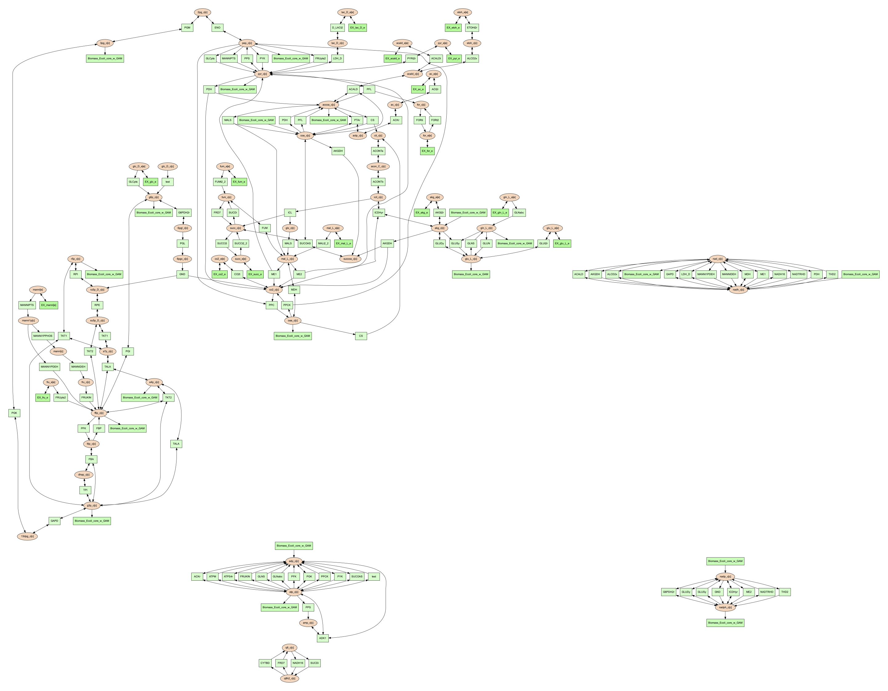
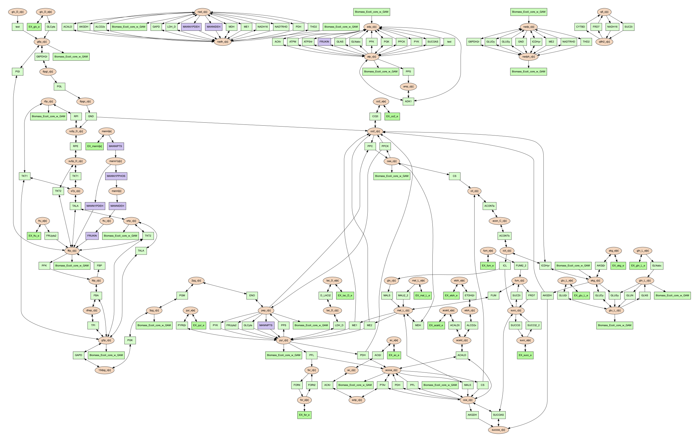
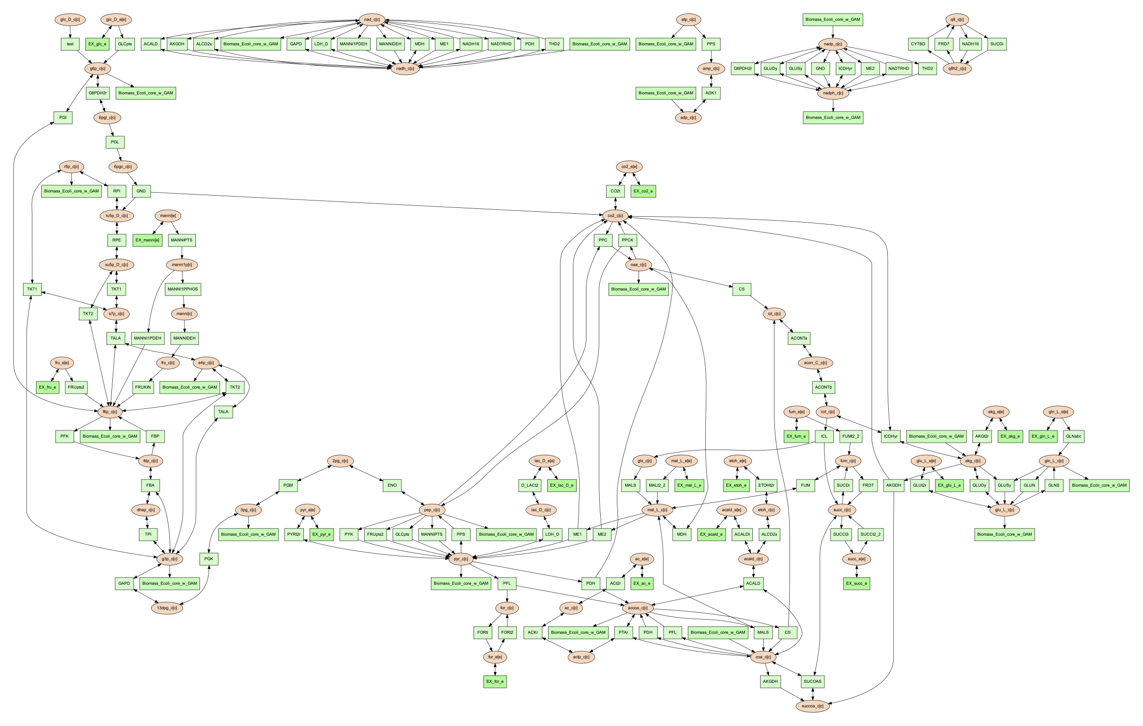
The commands above both generate an image file named ‘reactions.dot.pdf’. This pdf file is a graphical representation of what is in the ‘reactions.dot’. This graph will look like:

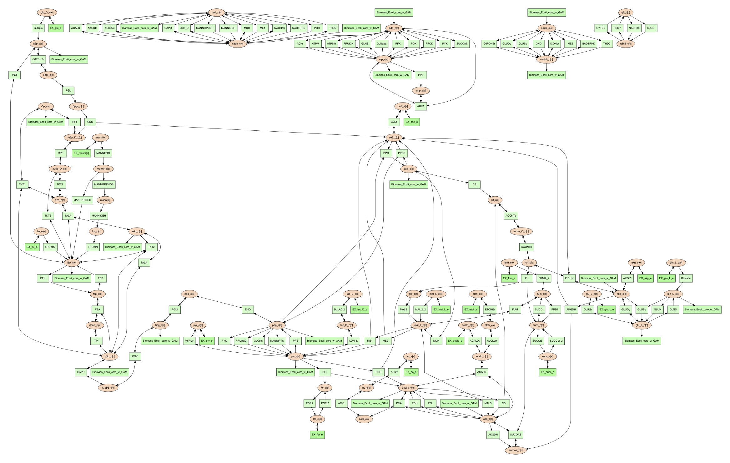
In this default version of the network image, there are two sets of nodes: oval orange nodes, which represent metabolites, and rectangular green nodes, which represent reactions. These nodes are connected by edges which indicate reaction directionality.

The rest of the tutorial will detail how to modify the default version of network image to show different aspects of the metabolism and customize the node properties. For these sections, the mannitol utilization pathway from the previous tutorial sections will be used as an example.

Represent Different Element Flows

By default, the vis command generates a graph that shows the carbon (C) transfer in the metabolic network. In the primarypairs tutorial section above, the element transfers in the ACKr reaction were examined to see how the FindPrimaryPairs algorithm would predict element transfer patterns. The vis command can use these element transfer predictions to filter edges in the network image, only edges that transfer specific element will be shown. In the case of the ACKr reaction, if element carbon is required to be shown, then only edges of ‘Acetate -> Acetyl-Phosphate’ and ‘ATP -> ADP’ would present in the final graph. The ‘ATP -> Acetyl-Phosphate’ edge will disappear, because ATP doesn’t transfer carbon to Acetyl-Phosphate.

Reactant/Product Pair	Element Transfer
Acetate -> Acetyl-Phosphate	carbon backbone
ATP -> ADP	carbon backbone, phosphates
ATP -> Acetyl-Phosphate	phosphate group
Acetate -> ADP	None

This type of element filtering can provide different views of the metabolic network by showing how metabolic pathways transfer different elements through those reactions. The mannitol utilization pathway is a multiple-step pathway that converts extracellular mannitol to fructose 6-phosphate. This pathway also involves multiple phosphorylation and dephosphorylation steps. The --element argument can be added to the the vis command to filter this pathway and show the transfer patterns of the phosphorus in the pathway:

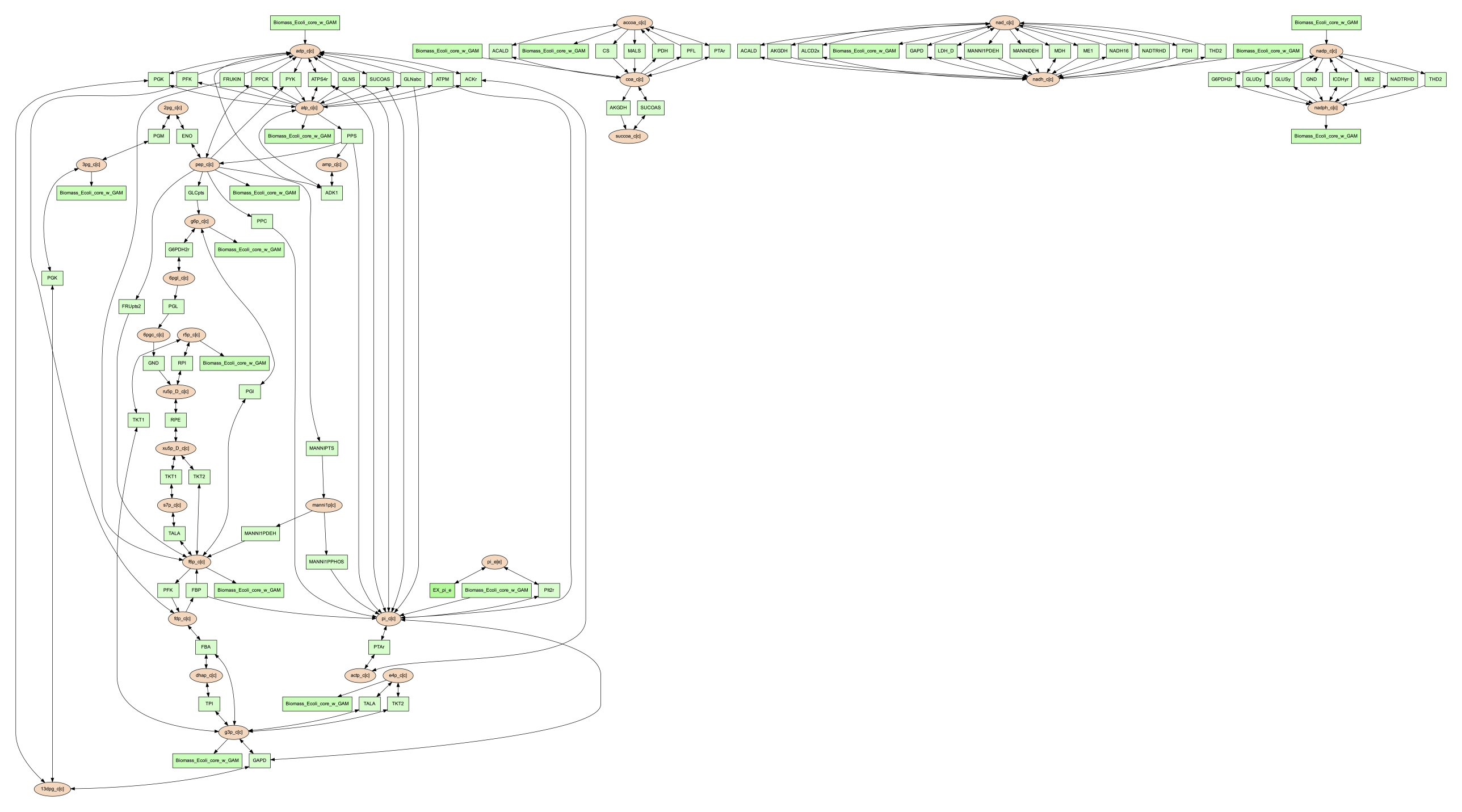
(psamm-model) $ psamm-model vis --element P --image png

The resulting ‘reactions.dot.png’ file will contain the phosphorus transfer network of the E. coli core model.

Condense Reaction Nodes and Edges

By default, the vis command assigns only one reaction to each reaction node. Additionally, it allows users to condense multiple reaction nodes into one node through the --combine option, in order to reduce the number of nodes and edges, and make the image clearer. Combine level 0 is the default, which does not collapse any nodes. Level 1 is used to condense nodes that represent the same reaction and have a common reactant or product connected. Level 2 is used to condense nodes that represent different reactions but connected to the same reactant/product pair with the same direction (This is often seen on reactant/product pairs like ATP/ADP and NAD/NADH).

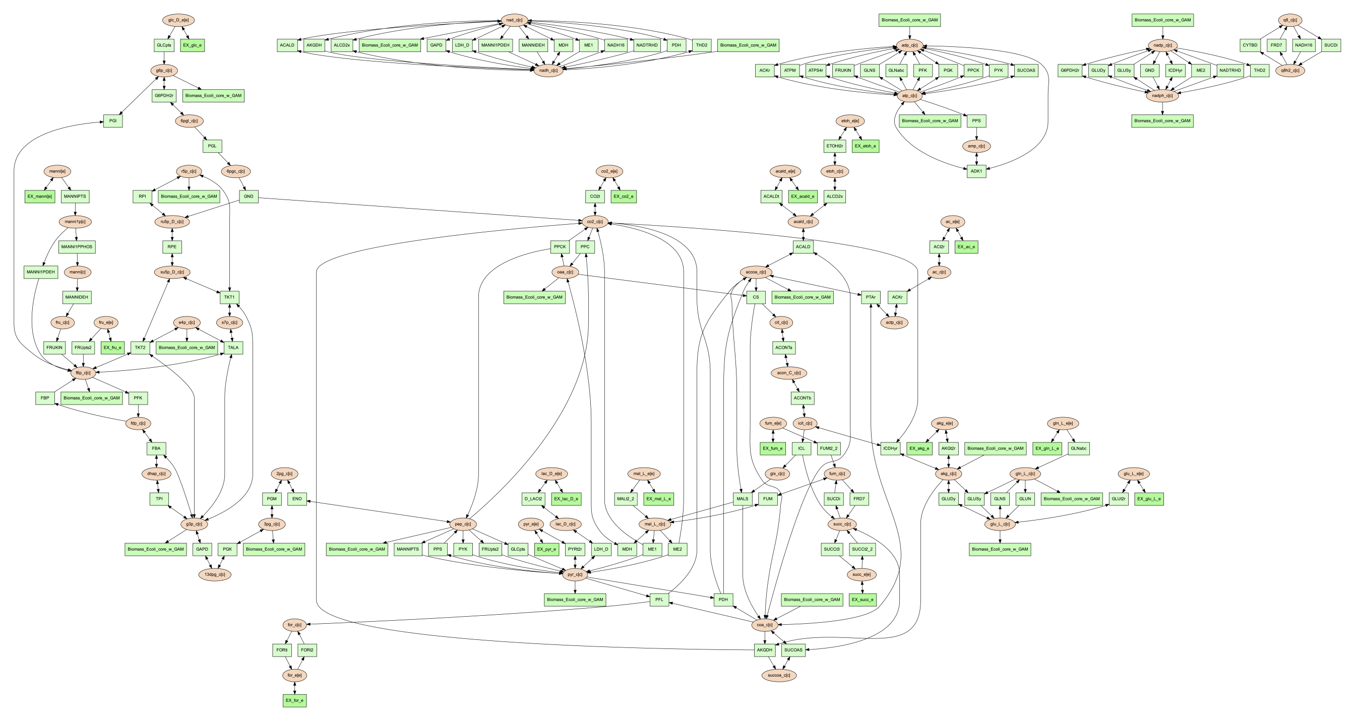
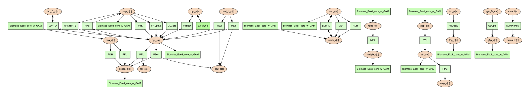
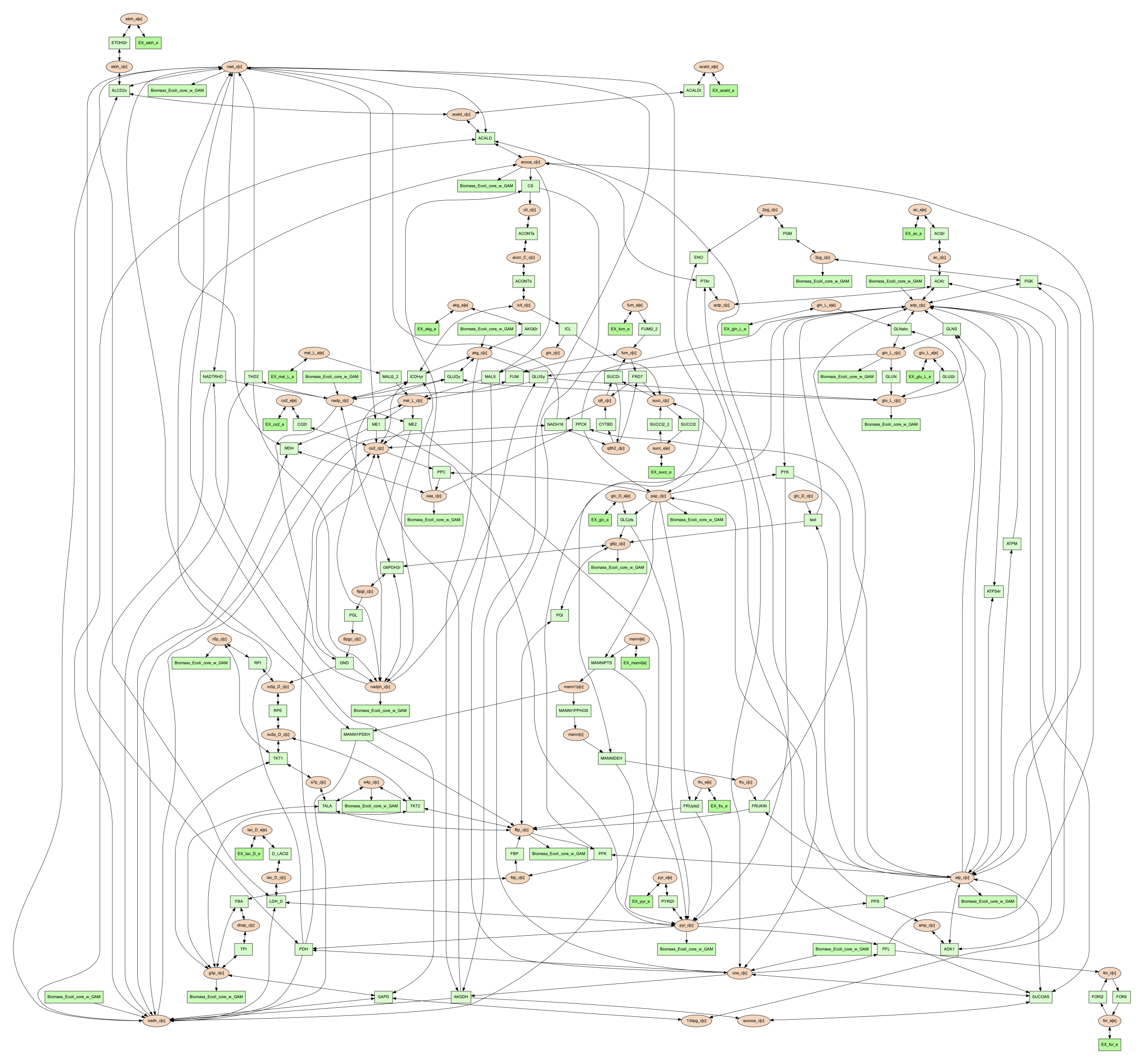
(psamm-env) $ psamm-model vis --combine 1 --image png

Then the image will look like the figure below:

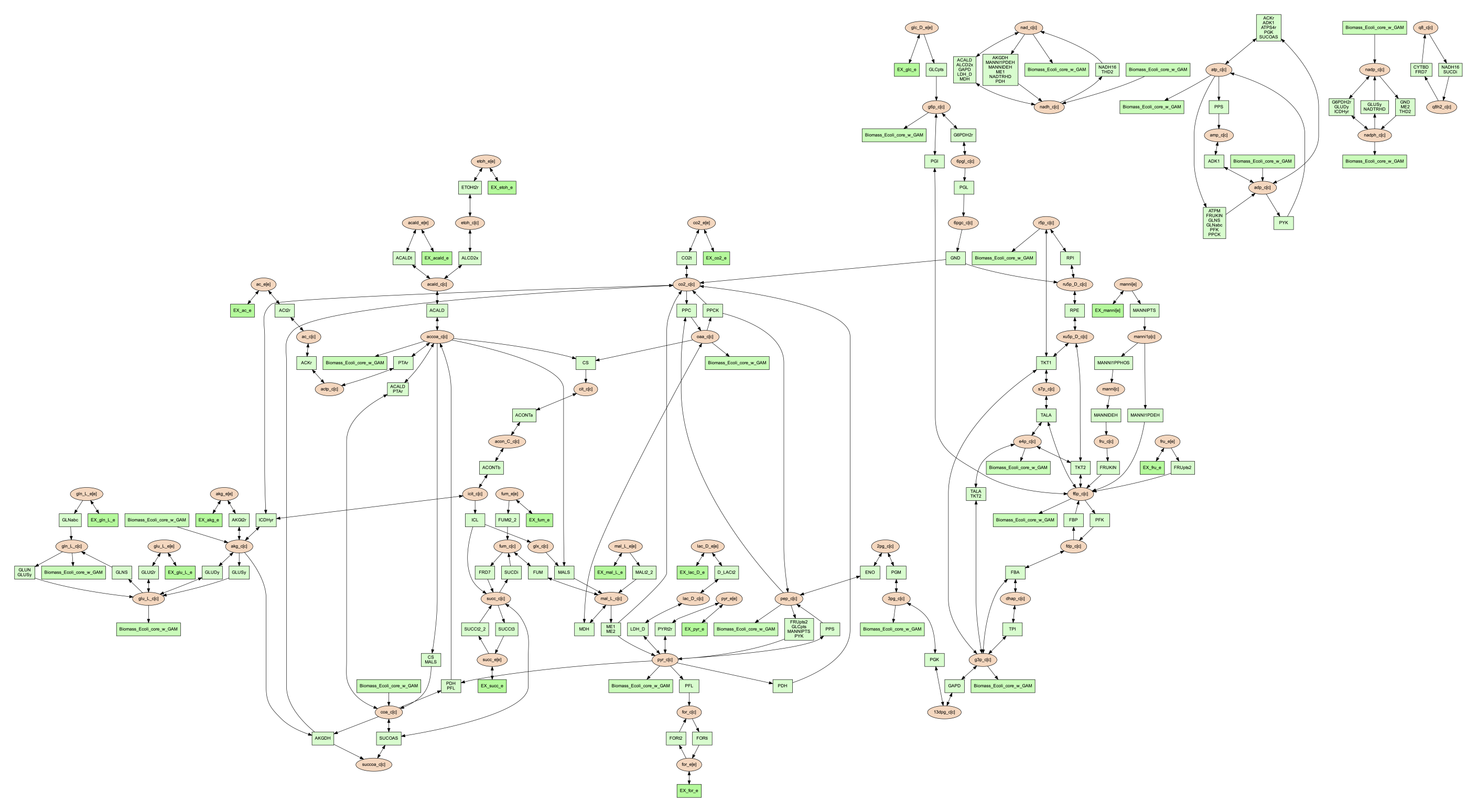
The combine 2 option will update the image to look like the following: .. code-block:: shell

(psamm-env) $ psamm-model vis –combine 2 –image png

Rearrange graph components in the image

In some cases, the network images contain many connected components, while these components aren’t connected with each other. This may cause the image too wide and difficult to read. To create a better view, --array option could be used. It can decompress graphs into their connected components, then arrange these components with specific array setting. --array is followed by an integer, for example, --array 2 indicates placing two connected components per row. For graphs that contains many small connected components, --array 4 could be a better option because you can get most of the important larger components in the top few rows of the image, and all the smaller components will just be spread out below them. Example of applying this option see below:

(psamm-env) $ psamm-model vis --image png --array 2

Then the exported image “reactions.dot.png” will look like the figure below:

Moreover, if vis command contains --array but doesn’t contain --image, it will still exported the DOT file. However, in this case, when converting DOT file to a network image, to make --array effective, another Graphviz program command (see below) is required instead of dot command we showed before:

(psamm-env) $ neato -O -Tpdf -n2 reactions.dot

Show Cellular Compartments

GEMs often contain some representations of cellular compartments. At the most basic level, this includes an intracellular and extracellular compartment, but in complex models, additional compartments such as the periplasm in bacteria or mitochondria in eukaryotes are often included. PSAMM-Vis can show these compartments in the final image through the use of the --compartment argument. If the compartment information is not defined in the model.yaml file, then, the command will attempt to automatically detect the organization of the compartments by examining the reaction equations in the model. However, this process cannot always accurately predict the compartment organization. To overcome this problem, it is suggested to define the compartment organization in the model.yaml file like in the following example:

name: Ecoli_core_model
biomass: Biomass_Ecoli_core_w_GAM
default_flux_limit: 1000
extracellular: e
compartments:
- id: c
  adjacent_to: e
  name: Cytoplasm
- id: e
  adjacent_to: e
  name: Extracellular
....

Once this information is added to the model.yaml file the following command can be used to generate an image that shows the compartment information of the model:

(psamm-env) $ psamm-model vis --compartment --image png

The resulting file ‘reactions.dot.png’ will look like the following:

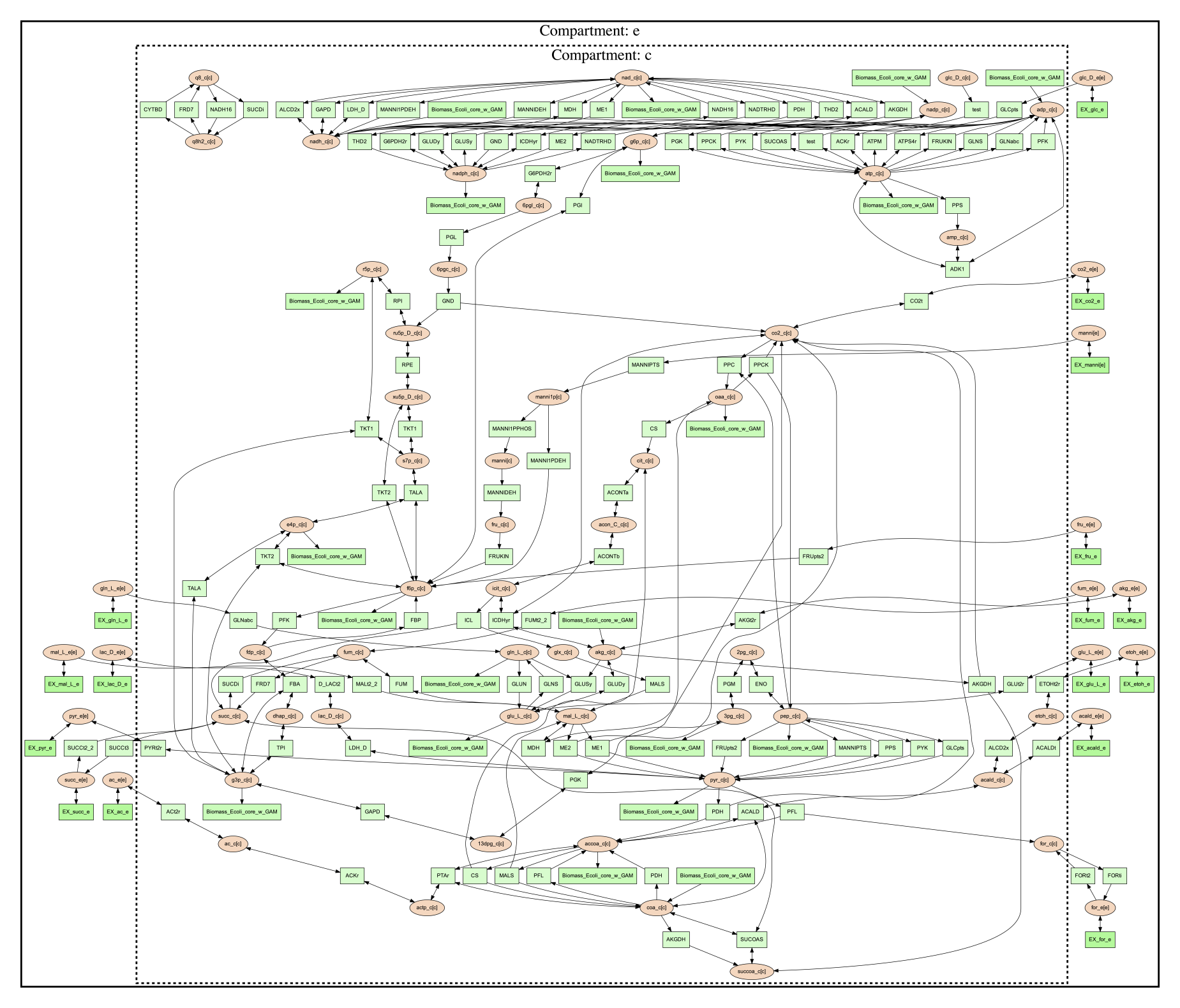
In this image there are two compartments that are labeled with ‘Compartment: e’ and ‘Compartment: c’. The E. coli core model is relatively small, meaning that compartment organization is simple, but vis command can handle more complex models as well. For example, the following image was made using a small example model to show a more complex compartments organization. To do this running the following command:

(psamm-env) $ psamm-model --model ../additional_files/toy_model_cpt/toy_model.yaml vis --image png --compartment

The resulting network image “reactions.dot.png” looks like:

Visualize Reactions and Pathways of Interest

In some situations, it might be better to visualize a subset of a larger model so that smaller subsystems can be examined in more detail. This can be done through the --subset option. This option takes an input of a single column file, where each line contains either a reaction ID or a metabolite ID. The whole file can contain only reaction IDs or metabolite IDs and cannot be a mix of both.

To show the usage of this option, a subset of reactions involved in mannitol utilization pathway was visualized through the following command:

(psamm-env) $ psamm-model vis --subset ../additional_files/subset_mannitol_pathway.tsv --image png

The input file subset_mannitol_pathway looks like the following:

MANNIPTS
MANNI1PDEH
MADNNIDEH
MANNII1PPHOS
FRUKIN

This resulting image “reactions.dot.png” looks like the following:

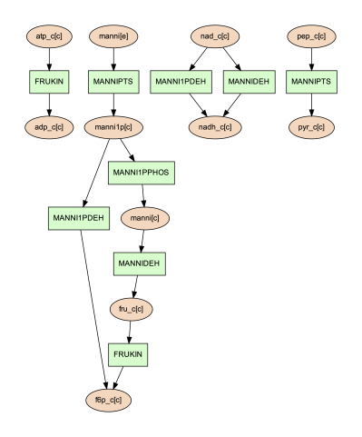
This image only contains reactions listed in the subset file and any associated exchange reactions.

The other usage for using the subset argument is to provide a list of metabolite IDs (with compartment). This option will generate an image containing all of the reactions that contain any of given metabolites in their equation. For example, the following subset file could be used to generate a network image of all reactions that contain pyruvate.

pyr_c[c]
pyr_e[e]

To use this subset to generate the pyruvate related subnetwork use the following command:

(psamm-env) $ psamm-model vis --subset ../additional_files/subset_pyruvate_list.tsv --image png

This will generate an image like the following that only shows the reactions that contain pyruvate:

Highlight Reactions and Metabolites in the Network

The --subset option can be used to show only a specific part of the network. When this is done, the context of those reactions is often lost and it can be hard to tell where that pathway fits within the larger metabolism. A different way to highlight a set of reactions without using the --subset option is to change the color of a set of nodes through the --color option.

This option can be used to change the color of the reaction or metabolite nodes on the final network image, making it easy to highlight certain pathways while still maintaining the larger metabolic context. This --color option will take a two-column file that contains reaction or metabolite IDs in the first column and hex color codes in the second column. A color file that can be used to color all of the mannitol utilization pathway reactions purple would look like the following:

MANNIPTS #d6c4f2
MANNI1PDEH #d6c4f2
MANNIDEH #d6c4f2
MANNI1PPHOS #d6c4f2
FRUKIN #d6c4f2

To use this file to generate an image of the larger network with the mannitol utilization pathway highlighted, use the following command:

(psamm-env) $ psamm-model vis --color ../additional_files/color_mannitol_pathway.tsv --image png

The resulting image file should look like the following:

Coloring of specific nodes like this can make it easy to locate or highlight specific pathways, especially in larger models.

Note

Reaction nodes that represent multiple reactions won’t be recolored even if it contains one or more reactions that are in input table for recolor.

Modify Node Labels in Network Images

By default, only the reaction IDs or metabolite IDs are shown on the nodes in final network images. These labels can be modified to include any additional information defined in the compounds or reactions YAML file through the use of the --cpd-detail and --rxn-detail options. These options are followed by a space separated list of metabolite or reaction property names, such as id, name, equation, and formula. The required properties will present on the node labels in network image. For example, for reaction ME1 (NAD-dependent malic enzyme), to show metabolite ID, name and formula, as well as reaction ID, and equation, running the following command:

(psamm-env) $ psamm-model vis --subset ../additional_files/detail_ME1.tsv --cpd-detail id name formula --rxn-detail id equation --image png

The image generated looks like this:

Note

For these two options, if a required detail is not included in the model, that property will be skipped and not shown on those nodes.

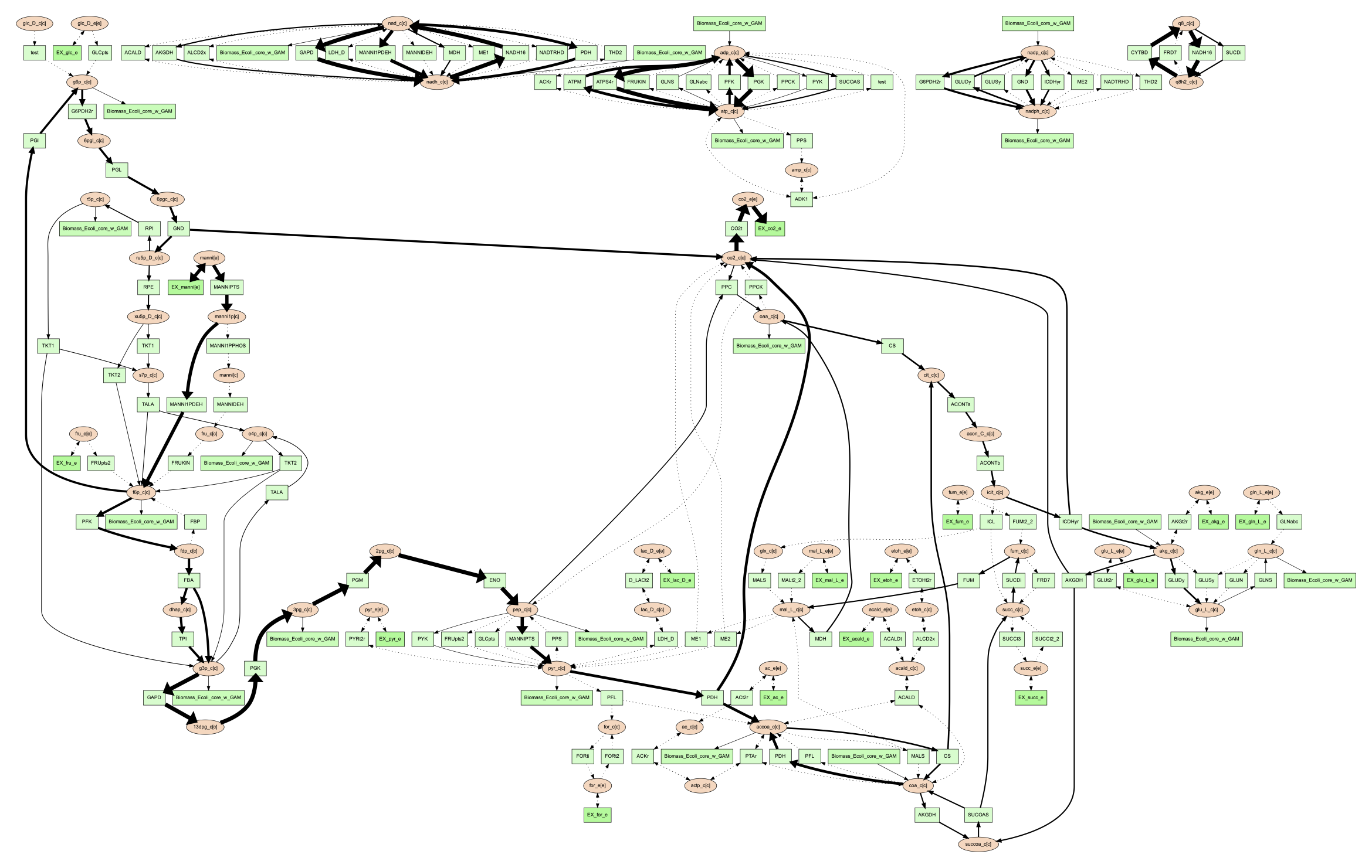
Visualize FBA or FVA

Performing various simulations of growth is made possible through methods such as FBA and FVA. Using the --fba or --fva option, the flow of metabolites calculated by these methods can be visualized. When visualizing FBA, a tsv file containing the reaction name and flux value is required. For example, the following command can be used:

(psamm-env) $ psamm-model vis --fba ../additional_files/fba.tsv --image png

The image generated looks like this:

If the FVA option is given, the file should contain the reaction name, and a lower and upper bound flux value that would still allow the model to sustain the same objective function flux. To visualize the FVA results, you can use the command:

(psamm-env) $ psamm-model vis --fva ../additional_files/fva.tsv --image png

The image generated looks like this:

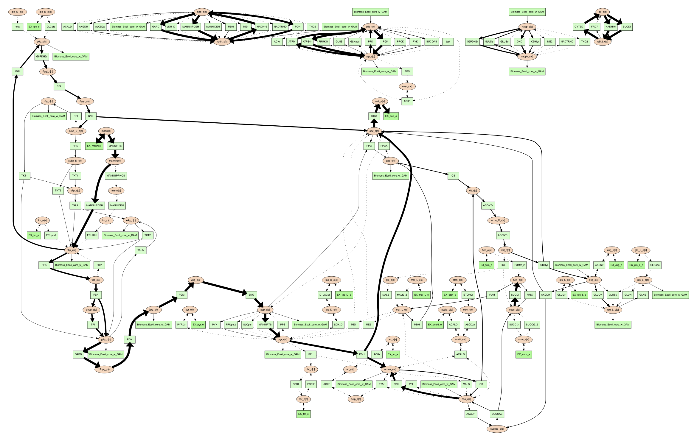
Reactions with a flux of zero is represented as a dotted edge and non-zero fluxes as solid. Meanwhile, the thickness of the edges is proportional to the flux through the reaction. Visualizing these fluxes may help highlight reactions that contribute the most to the objective.

Note

The --fba and --fva options cannot be used together.

Note

Fluxes less than the absolute value of 1e-5 will be considered as 0.

Other Visualization Options

Remove Specific Reactant Product Pairs

Large scale models may have some reactant/product pairs that occur many times in different reactions. These often involve currency metabolites like ATP, ADP, NAD and NADH. Due to the large number of times these pairs occur across the network, they may cause some parts of the graph to look messy. While making the condensed reaction nodes can help with this problem, there may be cases where it would be better to hide these edges in the final result. To do this the --hide-edges option can be used. This option takes a two-column file where each row contains two metabolite IDs separated by tab, edges between them will be hidden in final network image.

For example, to hide the edges between ATP and ADP in the E. coli core model, the input file would look like the following:

atp_c[c] adp_c[c]

Then the following command could be run to generate a network image that hides the edges between ATP and ADP:

(psamm-env) $ psamm-model vis --hide-edges ../additional_files/hide_edges_list.tsv --image png

When comparing this image to previous visualizations we can see that many edges between ATP and ADP have been removed from the graph. While this might not make a huge difference on a small model like this, on larger models this can help during the process of generating cleaner final images.

Adjusting Image Size

The size of the final network image generated through the vis command can be adjusted through the --image-size option. This option takes the width and height (in inches) separated by a space. The following command is an example that generates an image of 8.5 inches x 11 inches:

(psamm-env) $ psamm-model vis --image-size 8.5 11 --image png

The resulting image looks like:

Specifying A File Name

The vis command allows users to specify the directory and name of outputs through the --output option. This option should be followed by a string and this string is the full path with the prefix of outputs (without the file extension). For example, the following command will export 4 files in your current working directory : “Ecolicore.dot”, “Ecolicore.dot.png”, “Ecolicore.nodes.tsv” and “Ecolicore.edges.tsv”:

(psamm-env) $ psamm-model vis --image png --output Ecolicore

If you run the following two commands, you will get 4 files in the new folder named “test-output”: “Ecolicore.dot”, “Ecolicore.dot.png”, “Ecolicore.nodes.tsv” and “Ecolicore.edges.tsv”:

(psamm-env) $ mkdir test-output

(psamm-env) $ psamm-model vis --image png --output test-output/Ecolicore

Changing Pair Prediction Methods

By default, the vis function in PSAMM applies FindPrimaryPairs algorithm to predict reactant/product pairs. But it can also work without pair prediction (no-fpp). When``no-fpp`` is used, each reactant will be paired with all products in a reaction, without considering element transferred between reactant and product. There will tend to be many more connections in the network image if users use this option, especially for metabolites like ATP, H2O, and H+. To do this, running the following command:

(psamm-env) $ psamm-model vis --method no-fpp --image png

Note

The --method no-fpp and --combine options cannot be used together. The --combine option only works for FindPrimaryPairs method.